MScomplexes

Here, two case studies presenting how the pyms3d may be plugged into paraview are discussed. The first involves the Hydrogen dataset shown here . The second is the isabel case study and is shown using a video here .

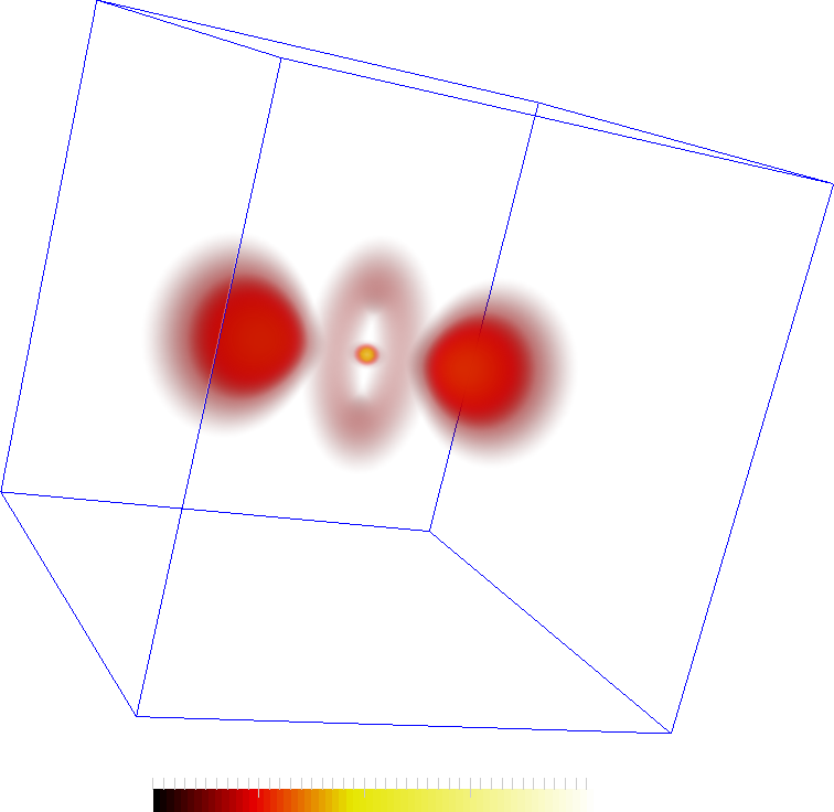
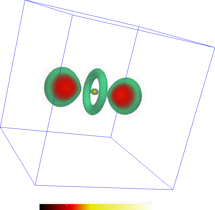
The hydrogen dataset is an EM scan of the hydrogen atom available from here . These images shows a simple voume rendering of the scalar values and features extracted from them. The second image also shows an iso-surface at 30. The features are the two lobes, central torus and a maximum in the center of the torus.

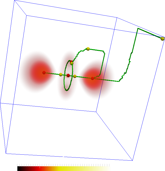
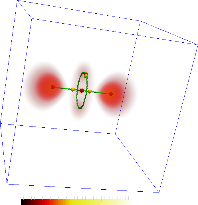
The features are represented by the maxima (red spheres) the following two images. The connectivity in the Morse-Smale complex captures the torus as well as the connectivity between the central lobes and the central maxima. However, not all connections may be interesting. In the second figure, two saddles are removed so that the remaining correspond more closely to the features in the dataset.

An important aspect is the programmable and interactive aspect of the design. The programmable aspect comes in handy when some filtering, such as those for the images above, is required.

The following are a pair of scripts that generate the geometry for the above visualizations. They are to be plugged into the paraview programmable source, and programmable filter respectively. The first script computes the Morse-Smale complex, simplifies it and then generates the geometry of the ascending manifolds of 2-saddles. The second generates the set of critical points that represent this geometry, namely the 2-saddles and the maxima they connect. In the first script, the set of saddles may be trimmed as desired. The line to do this is commented in the first script. It is uncommented to produce the fourth image above. As can be seen in both scripts, the code attempts to load data from a cache and only recomputes if it is unavailable.

The full paraview state file containing the pipeline necessary to generate the above images is available here . The raw float data (8Mb) is available here . Note: the scripts and the paraview state file assumes that the data is available in a folder named data. Edit that appropriately. Also, this was known to work with Paraview 4.3. In general, the Paraview Python API evolves quickly and the code may not work properly on earlier versions.

• Programmable Source to generate the 2-saddle geometry

  import pyms3d
  from paraview.vtk.numpy_interface import dataset_adapter as DA
  import numpy as np
  
  
  #data info
  DataFile = "data/Hydrogen_128x128x128.raw"
  Dim      = (128,128,128)
  
  # try to load from cache
  if hasattr(pyms3d,"msc") and hasattr(pyms3d,"pa"):
      msc  = pyms3d.msc
      pa   = pyms3d.pa
  else:
      # compute the mscomplex simplify and collect the 
      # ascending geometry of 2 saddles
      print pyms3d.get_hw_info()
      msc = pyms3d.mscomplex()
      msc.compute_bin(DataFile,Dim)
      msc.simplify_pers(thresh=0.05)
      msc.collect_geom(dim=2,dir=1)
      
  
      # the ascending geometry of 2-saddles is defined
      # on the dual grid. Get coorinates of dual points. 
      # i.e. The centroids of cubes
      dp = msc.dual_points()
      pa = vtk.vtkPoints()
      pa.SetData(DA.numpyTovtkDataArray(dp,"Pts"))
  
      # Cache objects
      setattr(pyms3d,"msc",msc)
      setattr(pyms3d,"pa",pa)
  
  #list of 2 saddle cps
  cps_2sad = msc.cps(2)
  #cps_2sad = [cps_2sad[i] for i in [0,1,3]]
  
  #put the list in cache 
  setattr(pyms3d,"cps_2sad",cps_2sad)
  
  # create a vtk CellArray for the line segments
  ca = vtk.vtkCellArray()
  for s in cps_2sad:
      gm = msc.asc_geom(s)
      for a,b in gm:
          ca.InsertNextCell(2)
          ca.InsertCellPoint(a)
          ca.InsertCellPoint(b)
  
  #Set the outputs
  pd = self.GetOutput()
  pd.SetPoints(pa)
  pd.SetLines(ca)
  

• Programmable Filter to extract the location of 2-saddles and maxima

  import pyms3d
  import numpy as np
  
  if hasattr(pyms3d,"msc") and hasattr(pyms3d,"cps_2sad"):
      msc      = pyms3d.msc
      cps_2sad = pyms3d.cps_2sad
  
      # create the list of 2-saddles and maxima locations
      cpList = []    
      for s in cps_2sad:
          cpList.append((msc.cp_cellid(s),2))
          for m,k in msc.asc(s):
              cpList.append((msc.cp_cellid(m),3))    
      cpList = list(set(cpList))        
      
      # create the vtk objects
      pa = vtk.vtkPoints()
      ia = vtk.vtkIntArray()
      ca = vtk.vtkCellArray()
      ia.SetName("Index")
  
      for i,(p,idx) in enumerate(cpList):
          pa.InsertNextPoint(np.array(p,np.float32)/2)
          ia.InsertNextValue(idx)
          ca.InsertNextCell(1)
          ca.InsertCellPoint(i)
  
      #Set the outputs
      pd = self.GetOutput()
      pd.SetPoints(pa)
      pd.SetCells(vtk.VTK_VERTEX,ca)
      pd.GetPointData().AddArray(ia)
  

Hurricane Isabel that struck the coast of Florida, USA, in September of 2003. A simulation of that event was made available here .

From this simulation, we extract the wind speed field of the 3D simulation volume. The eye of the hurricane is often a feature of interest. A typical feature of a hurricane is that the wind speeds are very low at the eye with very high speeds around it. This Video demonstrates how pyms3d can be used for segmentation and visual analysis.